Dynamical Critical Exponents in the 2D Ising Model
Critical slowing down makes equilibrium sampling progressively harder as a continuous transition is approached. At the Onsager point, the integrated autocorrelation time of the magnetization scales as
so the dynamical critical exponent \(z\) quantifies how fast the decorrelation cost grows with lattice size [1].
This notebook compares random-site Metropolis dynamics with the Wolff cluster update using the same measurement target as scripts/ising/measure_z.py. The central observable is the slope of \(\tau_{\mathrm{int}}(L)\) on log-log axes: Metropolis remains diffusion-limited (\(z \approx 2.17\)), while Wolff drastically reduces critical slowing down. In the cluster-step units used throughout this notebook, \(z^{\mathrm{cs}} \approx 0.5\) (asymptotic value; fits at
\(L = 16\)–\(128\) yield \(z^{\mathrm{cs}} \approx 0.40\)); normalised to equivalent-sweep units, \(z^{\mathrm{sw}} \approx 0.25\) [2, 3].
The analysis is organized in four parts:
Physical mechanism: why local and cluster dynamics produce different scaling slopes, and what the unit convention means.
Data ingestion: load cached script output (or run a small fallback demo).
Uncertainty-aware fitting: estimate \(z\) in log-log space with diagnostics and confidence intervals.
Interpretation: connect numerical slopes to sampling strategy and the difference between algorithmic efficiency and physical dynamics.
Why the slopes differ
Local Metropolis updates propose one spin-flip at a time, so relaxation near \(T_c\) is diffusive: the correlation length \(\xi\) diverges as the transition is approached, and the system must cross free-energy barriers through small local moves. This leads to \(z \approx 2.17\) for the 2D Ising random-site Metropolis [3].
Wolff instead grows a cluster from a random seed by bonding same-sign nearest neighbours with probability
a choice derived from the Fortuin–Kasteleyn random-cluster representation [4] that guarantees detailed balance with a 100% acceptance rate. Flipping a whole correlated domain in one move matches the scale of critical fluctuations and suppresses the diffusive bottleneck, yielding \(z^{\mathrm{cs}} \approx 0.5\) in cluster-step units [2, 3].
Defining \(\tau_{\mathrm{int}}\) and the update unit
\(\tau_{\mathrm{int}}\) counts the number of update steps required to generate one statistically independent sample. The meaning of “one step” differs between algorithms:
Algorithm |
Work per step |
|---|---|
Random-site Metropolis |
one spin-flip attempt |
Wolff cluster |
one cluster flip of \(\langle C \rangle\) spins — 100% acceptance rate |
Counting raw step numbers treats a Wolff step near \(T_c\) — which flips an \(O(L^{7/4})\)-spin cluster — as equivalent to a single Metropolis attempt. Comparing raw \(\tau_{\mathrm{int}}\) values directly is therefore misleading.
Normalisation to sweep-equivalent units
The standard fix is to express both algorithms in units of one \(L^2\)-flip-attempt sweep. Metropolis is already in this unit; Wolff requires reweighting by the mean cluster fraction:
At \(T_c\), the mean Wolff cluster size scales as \(\langle C \rangle \sim \chi \sim L^{\gamma/\nu} = L^{7/4}\), using the exact 2D Ising exponents \(\gamma = 7/4\) and \(\nu = 1\). Substituting into the sweep-equivalent relation:
With \(z^{\mathrm{cs}} \approx 0.5\), this gives \(z^{\mathrm{sw}} \approx 0.25\) — a 9× reduction relative to Metropolis, but not zero. Wolff drastically reduces critical slowing down; it does not eliminate it.
For the full work-normalisation derivation, ISS (independent-samples-per-second) comparison, and temperature-resolved data, see the companion Wolff Efficiency notebook.
Units used in this notebook
This notebook reports \(\tau_{\mathrm{int}}\) in cluster-step units throughout, matching the output of scripts/ising/measure_z.py. The measured Wolff slope is therefore the cluster-step exponent \(z^{\mathrm{cs}} \approx 0.5\) (asymptotic value; fits at \(L = 16\)–\(128\) yield \(z^{\mathrm{cs}} \approx 0.40\)). The sweep-equivalent exponent is \(z^{\mathrm{sw}} = z^{\mathrm{cs}} - 1/4 \approx 0.25\).
Load or compute data
This notebook needs \(\tau_{\mathrm{int}}(L)\) measurements at \(T_c\) for random-site Metropolis and Wolff updates across multiple lattice sizes. It first searches for precomputed results at ../results/ising/dynamic_exponent_z.npz.
If the cache exists, the notebook loads it directly. When per-size replicate arrays (tau_metro_samples, tau_wolff_samples) are present, medians are used as central values and 16–84% percentile bands are shown as error bars. If those fields are absent (legacy single-trajectory cache), the notebook still runs and treats each size as a single-point estimate with no error bars.
If the cache is missing, the notebook runs a small inline fallback (sizes 16, 24, 32 with short trajectories). The fallback is only for pipeline validation and quick plotting; it is not a publication-quality estimate of \(z\).
To generate high-quality cached data with uncertainty bands, run:
python scripts/ising/measure_z.py --sizes 16 32 48 64 96 128 --n-seeds 10
This writes ../results/ising/dynamic_exponent_z.npz with 10 independent seed replicas per (algorithm, \(L\)) point, matching the replication depth of the reference notebooks.
[1]:
from __future__ import annotations

import os

import matplotlib.pyplot as plt
import numpy as np

from utils.exceptions import ZeroVarianceAutocorrelationError
from utils.analysis import calculate_autocorr

TC_ISING = 2.0 / np.log(1.0 + np.sqrt(2.0))
NPZ_PATH = '../results/ising/dynamic_exponent_z.npz'
PALETTE = {'metro': '#4878CF', 'wolff': '#D65F5F'}


def estimate_tau(update: str, size: int, meas_steps: int, seed: int) -> float:
    from models.ising_model import IsingSimulation
    from utils.equilibration import convergence_equilibrate

    sim_r = IsingSimulation(size=size, temp=TC_ISING, update=update, init_state='random', seed=seed)
    sim_o = IsingSimulation(size=size, temp=TC_ISING, update=update, init_state='ordered', seed=seed)
    convergence_equilibrate(sim_r, sim_o, chunk_size=100, max_steps=10000)
    mags, _ = sim_r.run(n_steps=meas_steps)

    try:
        _, tau_int = calculate_autocorr(time_series=np.asarray(mags, dtype=float))
    except ZeroVarianceAutocorrelationError:
        tau_int = float('nan')

    return float(tau_int)


def _shape_to_samples(arr: np.ndarray) -> np.ndarray:
    """Return a 2D (n_size, n_rep) view for uncertainty handling."""
    a = np.asarray(arr, dtype=float)
    if a.ndim == 1:
        return a[:, None]
    return a


_cache_ok = False
if os.path.exists(NPZ_PATH):
    data = np.load(NPZ_PATH)
    required = {'L_metro', 'tau_metro', 'L_wolff', 'tau_wolff', 'Tc'}
    if required.issubset(set(data.files)):
        L_metro = np.asarray(data['L_metro'], dtype=float)
        tau_metro = np.asarray(data['tau_metro'], dtype=float)
        L_wolff = np.asarray(data['L_wolff'], dtype=float)
        tau_wolff = np.asarray(data['tau_wolff'], dtype=float)
        Tc = float(data['Tc'])

        # Optional replicate/sample arrays for uncertainty-aware aggregation.
        tau_metro_samples = _shape_to_samples(data['tau_metro_samples']) if 'tau_metro_samples' in data.files else tau_metro[:, None]
        tau_wolff_samples = _shape_to_samples(data['tau_wolff_samples']) if 'tau_wolff_samples' in data.files else tau_wolff[:, None]

        # Robust summary across replicates if available.
        tau_metro_med = np.nanmedian(tau_metro_samples, axis=1)
        tau_wolff_med = np.nanmedian(tau_wolff_samples, axis=1)
        tau_metro_p16 = np.nanpercentile(tau_metro_samples, 16, axis=1)
        tau_metro_p84 = np.nanpercentile(tau_metro_samples, 84, axis=1)
        tau_wolff_p16 = np.nanpercentile(tau_wolff_samples, 16, axis=1)
        tau_wolff_p84 = np.nanpercentile(tau_wolff_samples, 84, axis=1)

        n_rep_m = tau_metro_samples.shape[1]
        n_rep_w = tau_wolff_samples.shape[1]
        print(
            f'Loaded pre-computed data from {NPZ_PATH}: '
            f'{len(L_metro)} Metropolis sizes (replicates per size: {n_rep_m}), '
            f'{len(L_wolff)} Wolff sizes (replicates per size: {n_rep_w}).'
        )
        _cache_ok = True
    else:
        print(f'Cache at {NPZ_PATH} is missing expected keys; running inline fallback.')

if not _cache_ok:
    print(
        'Pre-computed data not found. Running inline demo '
        '(sizes 16, 24, 32; non-publication-quality).'
    )
    sizes = [16, 24, 32]
    L_metro = np.asarray(sizes, dtype=float)
    L_wolff = np.asarray(sizes, dtype=float)

    tau_metro = np.asarray(
        [estimate_tau(update='random', size=size, meas_steps=2500, seed=idx * 100) for idx, size in enumerate(sizes)],
        dtype=float,
    )
    tau_wolff = np.asarray(
        [estimate_tau(update='wolff', size=size, meas_steps=800, seed=idx * 100 + 1) for idx, size in enumerate(sizes)],
        dtype=float,
    )

    tau_metro_samples = tau_metro[:, None]
    tau_wolff_samples = tau_wolff[:, None]
    tau_metro_med = tau_metro.copy()
    tau_wolff_med = tau_wolff.copy()
    tau_metro_p16 = tau_metro.copy()
    tau_metro_p84 = tau_metro.copy()
    tau_wolff_p16 = tau_wolff.copy()
    tau_wolff_p84 = tau_wolff.copy()

    Tc = TC_ISING
    print(f'Computed fallback data at T_c = {Tc:.6f} for sizes {sizes}.')
Loaded pre-computed data from ../results/ising/dynamic_exponent_z.npz: 6 Metropolis sizes (replicates per size: 10), 6 Wolff sizes (replicates per size: 10).
Scaling fit with diagnostics and uncertainty
We fit the power law
by linear regression in log space:
where \(\tau_{\mathrm{int}}\) is the integrated autocorrelation time of the magnetization time series and \(A = A(T_c)\) is a non-universal prefactor.
Primary estimate: per-seed z distribution
With 10 independent seed replicas per \((L, \text{algorithm})\) point, the most direct way to quantify uncertainty in \(z\) is to fit independently for each seed and collect the resulting distribution:
The reported \(z\) and its 16–84% interval come from the median and percentiles of \(\{z_s\}\). This captures run-to-run variability in \(\tau_{\mathrm{int}}\) directly, rather than relying on OLS residuals over only six lattice sizes.
Reference curve: OLS fit on per-size medians
An OLS fit on the per-size median values provides a smooth reference line and 95% confidence band for the scaling plot. Per-size uncertainty is shown as error bars (16–84% across seeds at each \(L\)).
Both estimates are printed in the summary table below the figure.
[2]:
def fit_loglog(L: np.ndarray, tau: np.ndarray) -> dict[str, float | np.ndarray]:
    """Fit log(tau) = z*log(L) + b and return diagnostics."""
    valid = np.isfinite(L) & np.isfinite(tau) & (L > 0) & (tau > 0)
    x = np.log(np.asarray(L[valid], dtype=float))
    y = np.log(np.asarray(tau[valid], dtype=float))
    n = x.size
    if n < 3:
        raise ValueError('Need at least 3 valid points for log-log fit.')

    z, b = np.polyfit(x, y, 1)
    yhat = z * x + b
    resid = y - yhat
    rss = float(np.sum(resid**2))
    tss = float(np.sum((y - y.mean())**2))
    r2 = 1.0 - rss / tss if tss > 0 else np.nan

    sxx = float(np.sum((x - x.mean())**2))
    sigma2 = rss / (n - 2)
    z_se = float(np.sqrt(sigma2 / sxx))
    b_se = float(np.sqrt(sigma2 * (1.0 / n + (x.mean() ** 2) / sxx)))

    return {
        'z': float(z), 'b': float(b), 'A': float(np.exp(b)),
        'z_se': z_se, 'b_se': b_se, 'r2': float(r2),
        'x': x, 'y': y, 'yhat': yhat, 'resid': resid,
        'n': int(n), 'sigma': float(np.sqrt(sigma2)),
        'x_mean': float(x.mean()), 'sxx': sxx,
    }


def mean_band(fit: dict, x_new: np.ndarray) -> tuple[np.ndarray, np.ndarray, np.ndarray]:
    """OLS 95% confidence band for the mean log prediction, transformed to linear scale."""
    y_pred = fit['z'] * x_new + fit['b']
    se_mean = fit['sigma'] * np.sqrt(1.0 / fit['n'] + ((x_new - fit['x_mean']) ** 2) / fit['sxx'])
    return np.exp(y_pred), np.exp(y_pred - 1.96 * se_mean), np.exp(y_pred + 1.96 * se_mean)


# ---------------------------------------------------------------------------
# Per-seed z estimates: fit z independently for each replicate trajectory.
# This is the primary uncertainty estimate — it directly reflects run-to-run
# variability in tau_int rather than relying on OLS residuals over 6 sizes.
# ---------------------------------------------------------------------------
def _per_seed_z(L: np.ndarray, samples: np.ndarray) -> np.ndarray:
    """Return z fitted independently for each seed column in samples (n_size, n_seed)."""
    n_seeds = samples.shape[1]
    z_arr = np.full(n_seeds, np.nan)
    for s in range(n_seeds):
        col = samples[:, s]
        valid = np.isfinite(col) & (col > 0)
        if valid.sum() >= 3:
            z_arr[s] = fit_loglog(L[valid], col[valid])['z']
    return z_arr[np.isfinite(z_arr)]


z_seeds_m = _per_seed_z(L_metro, tau_metro_samples)
z_seeds_w = _per_seed_z(L_wolff, tau_wolff_samples)

z_m_med  = float(np.median(z_seeds_m))
z_w_med  = float(np.median(z_seeds_w))
z_m_p16, z_m_p84 = float(np.percentile(z_seeds_m, 16)), float(np.percentile(z_seeds_m, 84))
z_w_p16, z_w_p84 = float(np.percentile(z_seeds_w, 16)), float(np.percentile(z_seeds_w, 84))

# OLS fit on the per-size medians: used for the reference curve and CI band only.
fit_m = fit_loglog(L_metro, tau_metro_med)
fit_w = fit_loglog(L_wolff, tau_wolff_med)

L_fit = np.linspace(min(np.min(L_metro), np.min(L_wolff)),
                    max(np.max(L_metro), np.max(L_wolff)), 300)
tau_fit_m, tau_fit_m_lo, tau_fit_m_hi = mean_band(fit_m, np.log(L_fit))
tau_fit_w, tau_fit_w_lo, tau_fit_w_hi = mean_band(fit_w, np.log(L_fit))

# ---------------------------------------------------------------------------
# Figure: Left — scaling plot with seed uncertainty bands.
#         Right — per-seed z distributions (the primary uncertainty view).
# ---------------------------------------------------------------------------
fig, axes = plt.subplots(1, 2, figsize=(13, 5))

# --- Left panel: tau_int(L) scaling ---
ax = axes[0]
yerr_m = np.vstack([tau_metro_med - tau_metro_p16, tau_metro_p84 - tau_metro_med])
yerr_w = np.vstack([tau_wolff_med - tau_wolff_p16, tau_wolff_p84 - tau_wolff_med])

ax.errorbar(L_metro, tau_metro_med, yerr=yerr_m,
            fmt='o', color=PALETTE['metro'], markersize=6, capsize=3,
            label=f'Metropolis  $z = {z_m_med:.2f}$ [{z_m_p16:.2f}, {z_m_p84:.2f}]')
ax.errorbar(L_wolff, tau_wolff_med, yerr=yerr_w,
            fmt='s', color=PALETTE['wolff'], markersize=6, capsize=3,
            label=f'Wolff (cs)  $z = {z_w_med:.2f}$ [{z_w_p16:.2f}, {z_w_p84:.2f}]')

ax.loglog(L_fit, tau_fit_m, '--', color=PALETTE['metro'], alpha=0.9)
ax.loglog(L_fit, tau_fit_w, '--', color=PALETTE['wolff'], alpha=0.9)
ax.fill_between(L_fit, tau_fit_m_lo, tau_fit_m_hi, color=PALETTE['metro'], alpha=0.15)
ax.fill_between(L_fit, tau_fit_w_lo, tau_fit_w_hi, color=PALETTE['wolff'], alpha=0.15)

ax.set_xlabel('Lattice size $L$')
ax.set_ylabel(r'Integrated autocorrelation time $\tau_{\mathrm{int}}$')
ax.set_title(fr'Scaling at $T_c \approx {Tc:.4f}$  (error bars: 16–84% over seeds)')
ax.legend(fontsize=9, title='16–84% from per-seed z', title_fontsize=8)
ax.grid(True, which='both', alpha=0.25)

# --- Right panel: per-seed z distributions ---
ax = axes[1]
n_m = len(z_seeds_m)
n_w = len(z_seeds_w)

rng = np.random.default_rng(42)
jitter_m = rng.uniform(-0.15, 0.15, n_m)
jitter_w = rng.uniform(-0.15, 0.15, n_w)

ax.scatter(np.ones(n_m) + jitter_m, z_seeds_m,
           color=PALETTE['metro'], alpha=0.6, s=30, zorder=3)
ax.scatter(2 * np.ones(n_w) + jitter_w, z_seeds_w,
           color=PALETTE['wolff'], alpha=0.6, s=30, zorder=3)

for x_pos, med, p16, p84, col in [
    (1, z_m_med, z_m_p16, z_m_p84, PALETTE['metro']),
    (2, z_w_med, z_w_p16, z_w_p84, PALETTE['wolff']),
]:
    ax.plot([x_pos - 0.25, x_pos + 0.25], [med, med], '-', color=col, lw=2.5, zorder=4)
    ax.plot([x_pos, x_pos], [p16, p84], '-', color=col, lw=1.5, alpha=0.7, zorder=4)

ax.set_xticks([1, 2])
ax.set_xticklabels(['Metropolis', 'Wolff (cluster-step)'])
ax.set_ylabel('Fitted dynamical exponent $z$')
ax.set_title(f'Per-seed $z$ distribution  ({n_m} Metro, {n_w} Wolff seeds)')
ax.grid(axis='y', alpha=0.25)
ax.set_xlim(0.5, 2.5)

fig.tight_layout()
plt.show()

# ---------------------------------------------------------------------------
# Summary table
# ---------------------------------------------------------------------------
print('z from per-seed fit distribution (primary estimate):')
print('-' * 70)
print(f'  Metropolis     z = {z_m_med:.3f}  (16–84%: {z_m_p16:.3f} – {z_m_p84:.3f})  n_seeds = {n_m}')
print(f'  Wolff (cs)     z = {z_w_med:.3f}  (16–84%: {z_w_p16:.3f} – {z_w_p84:.3f})  n_seeds = {n_w}')
print()
print('OLS fit on per-size medians (reference line on left panel):')
print('-' * 70)
print(f"  Metropolis     z = {fit_m['z']:.3f}  (OLS SE: {fit_m['z_se']:.3f},  R² = {fit_m['r2']:.4f})")
print(f"  Wolff (cs)     z = {fit_w['z']:.3f}  (OLS SE: {fit_w['z_se']:.3f},  R² = {fit_w['r2']:.4f})")
print()
print('Note: Wolff z is in cluster-step units; sweep-equivalent z ≈ z_cs − 0.25.')
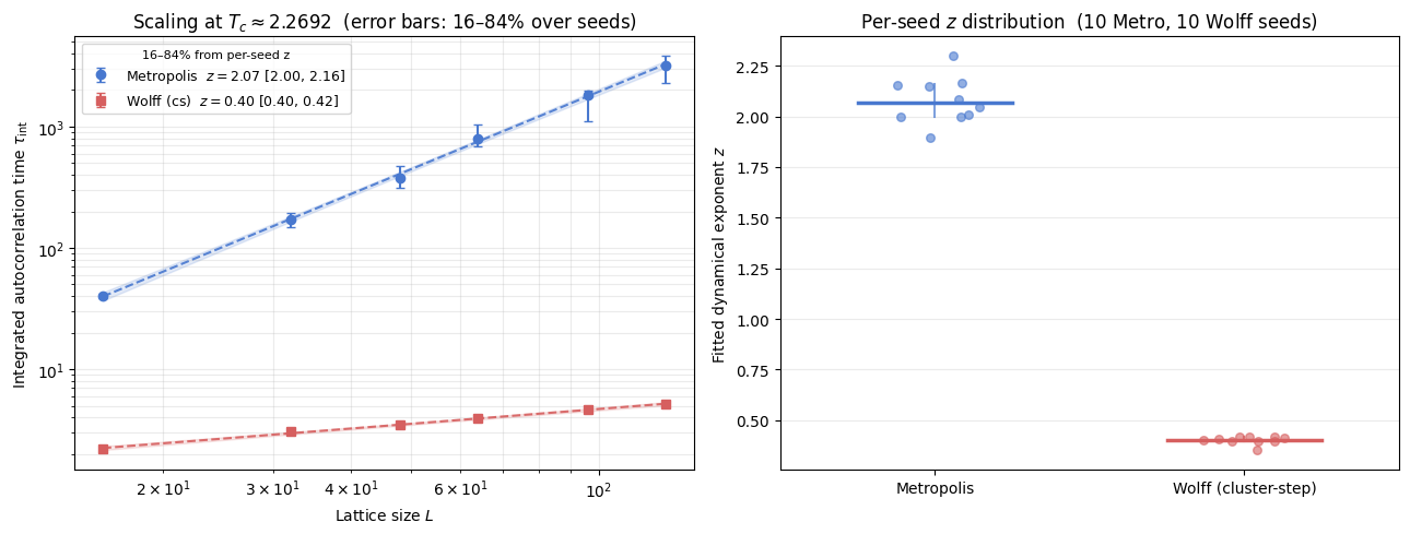
z from per-seed fit distribution (primary estimate):
----------------------------------------------------------------------
  Metropolis     z = 2.065  (16–84%: 1.998 – 2.161)  n_seeds = 10
  Wolff (cs)     z = 0.405  (16–84%: 0.397 – 0.416)  n_seeds = 10

OLS fit on per-size medians (reference line on left panel):
----------------------------------------------------------------------
  Metropolis     z = 2.119  (OLS SE: 0.030,  R² = 0.9992)
  Wolff (cs)     z = 0.404  (OLS SE: 0.014,  R² = 0.9954)

Note: Wolff z is in cluster-step units; sweep-equivalent z ≈ z_cs − 0.25.
Reading the result
The core signal is the separation of slopes:
Metropolis remains near the textbook local-dynamics regime (\(z \approx 2.17\)).
Wolff (in cluster-step units) yields a slope \(z^{\mathrm{cs}} \approx 0.40\) at these system sizes (\(L = 16\)–\(128\)), approaching the asymptotic value \(z^{\mathrm{cs}} \approx 0.5\) as \(L \to \infty\). This indicates that cluster updates change the scaling law rather than only reducing a prefactor.
Unit interpretation. The Wolff slope reported here is the cluster-step exponent \(z^{\mathrm{cs}}\). In sweep-equivalent units the normalised exponent is
which follows from \(\langle C \rangle \sim L^{\gamma/\nu} = L^{7/4}\) (exact 2D Ising FK scaling). This is roughly 9× smaller than the Metropolis exponent — a dramatic reduction, though not complete elimination of critical slowing down. For a full normalised comparison see the Wolff Efficiency notebook.
Use the confidence intervals as stability diagnostics, not as strict final error bars, because finite-size windows and replicate counts in the cache can differ across runs. The right panel shows the per-seed \(z\) distribution; a tight cluster near the median indicates a stable power-law regime over the measured \(L\) range.
Scientific implication
For equilibrium sampling near criticality, Wolff is generally the right algorithmic choice because it suppresses critical slowing down while preserving the Boltzmann target distribution.
However, a smaller algorithmic \(z\) does not mean Wolff reproduces physical kinetic time. For non-equilibrium kinetics and dynamic universality studies tied to local physical updates, random-site Metropolis (or another local dynamics) remains the physically interpretable model, even when it is computationally slower.
Bibliography
[1] L. Onsager, “Crystal Statistics. I. A Two-Dimensional Model with an Order-Disorder Transition,” Physical Review, vol. 65, no. 3-4, pp. 117-149, 1944. APS Open Access
[2] U. Wolff, “Collective Monte Carlo Updating for Spin Systems,” Physical Review Letters, vol. 62, no. 4, pp. 361-364, 1989. APS Open Access
[3] A. D. Sokal, “Monte Carlo Methods in Statistical Mechanics: Foundations and New Algorithms,” lecture notes (1989), published in Functional Integration: Basics and Applications (C. DeWitt-Morette, P. Cartier, A. Folacci, eds.), Springer, 1997, pp. 131-192. Standard reference for integrated autocorrelation-time estimators and error analysis in Markov-chain Monte Carlo. Springer Link
[4] C. M. Fortuin and P. W. Kasteleyn, “On the random-cluster model. I. Introduction and relation to other models,” Physica, vol. 57, no. 4, pp. 536-564, 1972. Original paper introducing the random-cluster (FK) representation that underpins the Wolff and Swendsen–Wang algorithms. Elsevier Open Access